Flow Loss Coefficient For a Round Pipe With Non-Uniform Roughness
\( \mathrm{Re} \gt 2000 \)
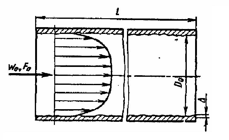
- \( w_0\) - mean flow velocity
- \( F_0\) - cross-sectional area
- \( D_0\) - internal diameter of pipe
- \( \ell\) - length of pipe
- \( \Delta\) - absolute surface roughness
- \( \bar{\Delta} = \Delta/D_0\) - relative surface roughness
Pipes with non-uniform or practical roughness represent real-world conditions in systems like wastewater lines, storm sewers, and aging infrastructure. These pipes may include corrosion pits, scale buildup, joint misalignments, and manufacturing defects that disrupt flow.
This page helps estimate pressure losses using flow loss coefficients (K-factors) tailored to irregular surfaces. Most pipes, tubes, and channels of engineering interest have uneven or non-uniform surface roughness. Flow loss coefficient depends on the relative surface roughness and Reynolds number.
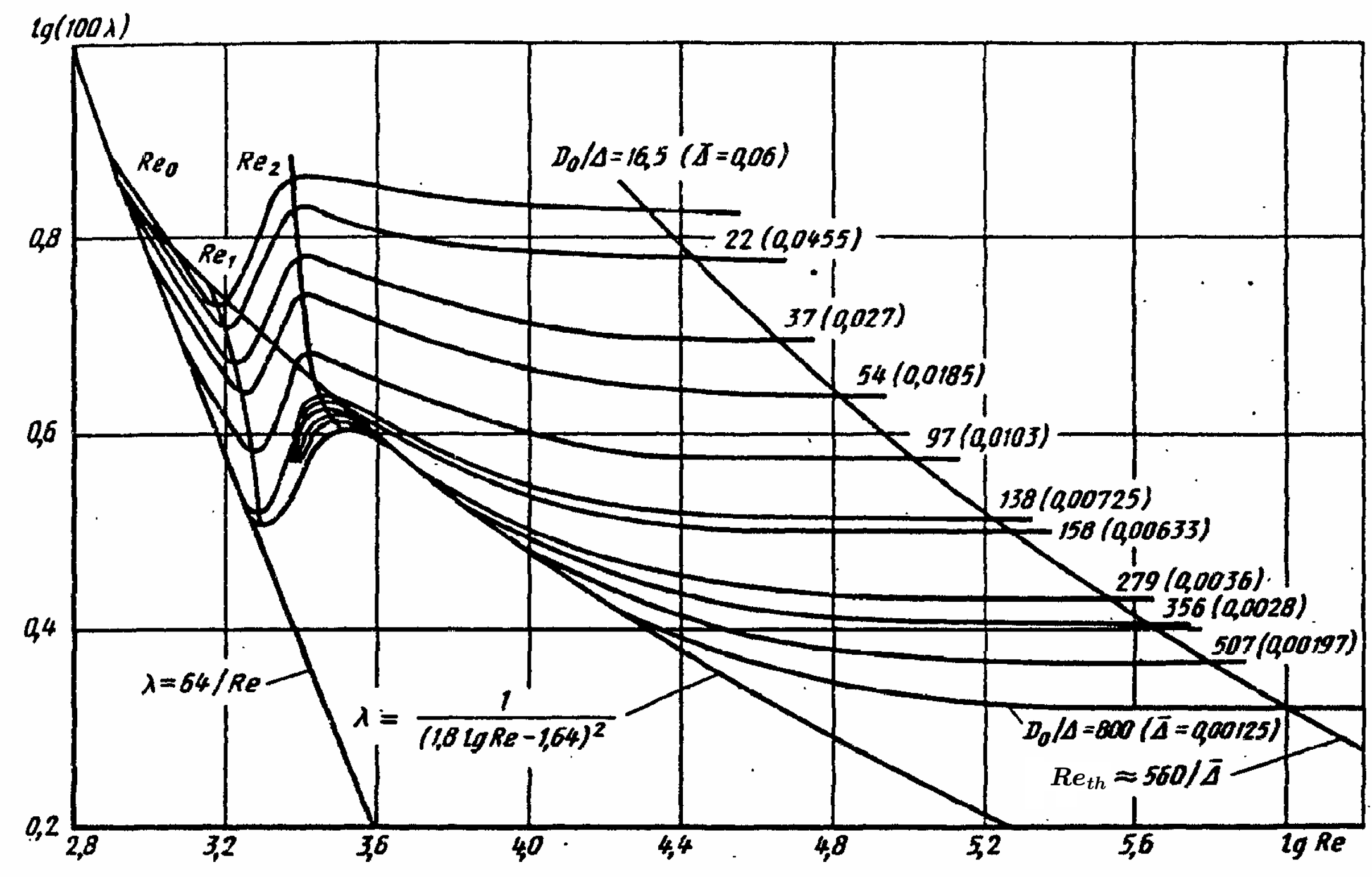
For pipes with equivalent roughness \( \bar{\Delta} > 0.007 \), flow coefficient curves deviate from Hagen-Poiseuille solution \( \lambda=64/\mathrm{Re}\); \( \lambda \) is larger than laminar solution for a given \( \mathrm{Re} \). The greater the relative surface roughness, the sooner this deviation occurs at \( \mathrm{Re_0} \):
$$ \mathrm{Re_0} = 754\exp{\left(\frac{0.0065}{\bar{\Delta}}\right)}$$
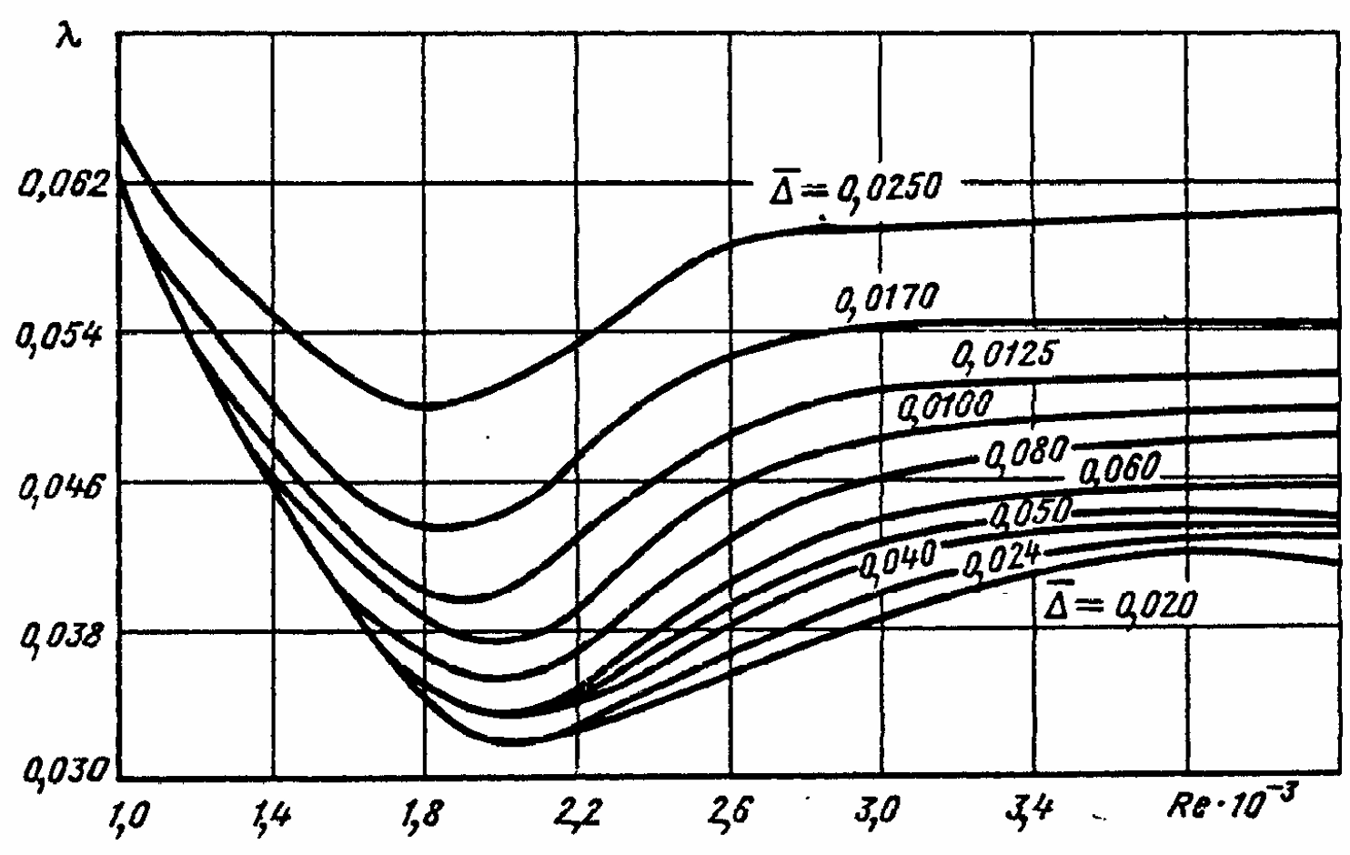
Flow coefficient in transition from laminar to turbulent flow regime depends on \( \bar{\Delta} \). Unlike flow with uniform sand grain roughness, there exists a unique curve for each \( \bar{\Delta} \) between \( \mathrm{Re_1} \) and \( \mathrm{Re_2} \):
$$ \mathrm{Re_1} = 1160 \left(\frac{1}{\bar{\Delta}}\right)^{0.11}$$
$$ \mathrm{Re_2} = 2090 \left(\frac{1}{\bar{\Delta}}\right)^{0.0635}$$
For \( \mathrm{Re} > \mathrm{Re_2} \), pipes and channels with uneven surface roughness can be treated as hydraulically smooth (within 3-4%) if \( \Delta \lt \bar{\Delta}_{th} \approx 15/\mathrm{Re} \). In other words, the flow loss coefficient traces \( \lambda = 1/(1.8 \log_{10}{\mathrm{Re}}-1.64)^2 \) curve between \( \mathrm{Re_2} \) and \( \mathrm{Re_{smooth}}\). Hence, pipes stop being hydraulically smooth at:
$$ \mathrm{Re_smooth} \approx \frac{15}{\bar{\Delta}}$$
Quadratic law of resistance for which \( \lambda \) remains constant starts, within 3-4%, at \( \mathrm{Re_{th}}\):
$$ \mathrm{Re_th} \approx \frac{560}{\bar{\Delta}}$$
For \( \mathrm{Re_0} \lt \mathrm{Re} \lt \mathrm{Re_1} \) and \( \bar{\Delta} \ge 0.007 \):
$$ \lambda = 4.4 \mathrm{Re}^{-0.595} \exp{\left( -\frac{0.00275}{\bar{\Delta}} \right)}$$
For \( \mathrm{Re_1} \lt \mathrm{Re} \lt \mathrm{Re_2} \):
$$ \lambda = (\lambda_2 - \lambda^*) \exp{\left( -\left[ 0.0017(\mathrm{Re_2}-\mathrm{Re})\right]^2 \right) + \lambda^*}$$
where:
| \( \bar{\Delta} \le 0.007 \) | \( \bar{\Delta} \gt 0.007 \) |
|---|---|
| \( \lambda^* = \lambda_1 \) | \( \lambda^* = \lambda_1 -0.0017 \) |
| \( \lambda_1 \approx 0.0032\) | \( \lambda_1 = 0.0775 - \frac{0.0109}{\bar{\Delta}^{0.286}} \) |
| \( \lambda_2 = 7.224(\mathrm{Re_2})^{-0.643}\) | \( \lambda_2 = \frac{0.145}{\bar{\Delta}^{-0.244}} \) |
| \( \mathrm{Re_0} = 2000 \) | \( \mathrm{Re_0} = 754\exp{\left(\frac{0.0065}{\bar{\Delta}}\right)} \) |
| \( \mathrm{Re_1} = 2000 \) | \( \mathrm{Re_1} = 1160 \left(\frac{1}{\bar{\Delta}}\right)^{0.11} \) |
| \( \mathrm{Re_2} = 2090 \left(\frac{1}{\bar{\Delta}}\right)^{0.0635} \) | \( \mathrm{Re_2} = 2090 \left(\frac{1}{\bar{\Delta}}\right)^{0.0635} \) |
For \( \mathrm{Re} \gt \mathrm{Re_2} \), can use implicit Colebrooke-White equation:
$$ \lambda = \frac{1}{\left[ 2\log_{10}{\left( \frac{2.51}{\mathrm{Re}\sqrt{\lambda}} +\frac{\bar{\Delta}}{3.7} \right)} \right]^2}$$
For engineering applications, the following approximation can be used:
$$ \lambda = 0.11 \left( \bar{\Delta} + \frac{68}{\mathrm{Re}} \right)^{0.25} $$
